Simulation Building Blocks

SimCADO objects

Source

The Source class is probably the most important class for testing science cases. Therefore spending time on creating accurate Source representations of the object of interest is key to getting good results with SimCADO.

Basically a Source object represents photon sources using lists of positions (.x, .y), a list of unique spectra (.spectra) and a list of references which match each photon source to a spectrum in the list of spectra (.ref). All sources (extended and point source) can be decomposed into these lists. The advantage of using this approach is that objects with highly similar spectra can both reference the same position in .spectra, thereby reducing the number of spectra that need to be manipulated during a simulation.

File Format of saved Source objects

Source objects are stored as FITS files with 2 extensions. The first (ext=0) contains an image with dimensions (n, 4) where n is the number of positions for which there exists a spectrum - i.e. non-empty space. The 4 rows of the image correspond to the .x, .y, .ref, .weight arrays. The second extension (ext=1) contains another image with dimensions (m+1, len(lam)), where m is the number of unique spectra and len(lam) is the length of the .lam array containing the centres of all wavelength bins. The first row in the second extension is the .lam array.

Todo

describe how Source is linked to OpticalTrain, Detector and UserCommands

OpticalTrain

Todo

describe how OpticalTrain is linked to Source, Detector and UserCommands

Detector

Todo

describe how Detector is linked to Source, OpticalTrain and UserCommands

UserCommands

Todo

descript how UserCommands is linked to Source, OpticalTrain and Detector

SimCADO methods

Method behind applying an OpticalTrain to a Source object

(Taken from Leschinski et al. 2016)

In an ideal world, SimCADO would apply all spectral and spatial changes at the resolution of the input data. However, the memory requirements to do this are well outside the limits of a personal computer. The solution to this problem is to split the effects based on dimensionality. For certain elements in the optical train, the spectral and spatial effects can be decoupled (e.g. purely transmissive elements like the filters versus purely spatial effects like telescope vibration). For other elements, most notably the PSF and ADC, all three dimensions must be considered simultaneously. When applying an OpticalTrain, SimCADO follows the procedure described graphically in Figure 1. The example used in Figure 1 is for a simplified stellar cluster with only two different stellar types - A0V and K5V type stars.

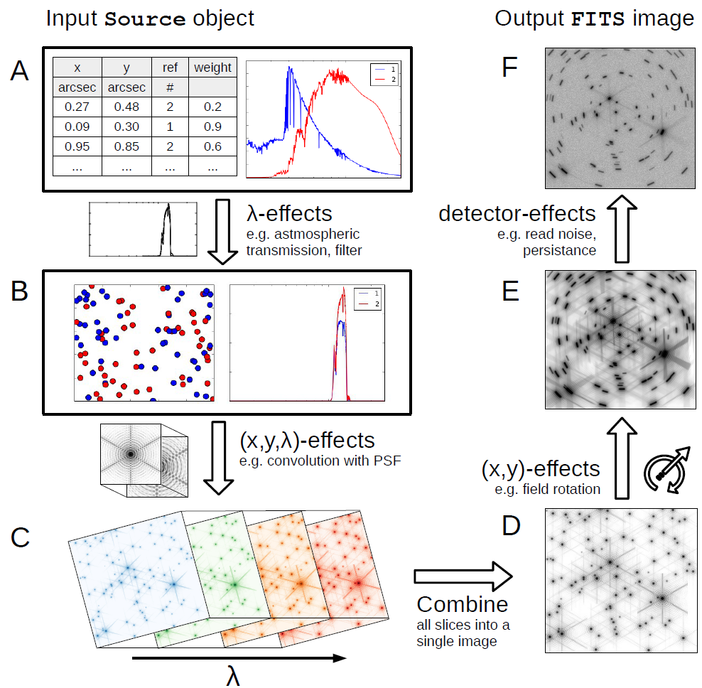
Figure 1 - The steps involved in applying an OpticalTrain object to a Source object. The example used here is for a simplified stellar cluster with only two different stellar types - A0V and K5V type stars.

• A. The original Source object includes an array of spectra for each unique photon source (in the case of Figure 1, there are only two unique spectra) and four vectors: x, y, ref, weight. x and y hold the spatial information for each photon source, ref connects each source to a spectrum in the array of spectra and weight allows the spectrum to be scaled.

• Spectral-effects. The first step in apply_optical_train() is to combine all optical elements which only act in the wavelength domain (e.g. filters, mirrors, etc.) into a single effect, then apply that effect to the array of spectra in the Source object.

• B. The spectra in the Source object are now representative of the photo-electron count at the detector, assuming a perfect optical train and at the internal spatial resolution of the simulation, i.e. not at the pixel scale of the detector. The position vectors are converted into a two-dimensional “image” of the Source.

• Spectrospatial-effects. The second step includes creating “slices” through the data. The spectra are binned according to several criteria (ADC shift, PSF FWHM difference, etc) with a spectral resolution anywhere from R=1 to R>100, and the number of photons per source in each wavelength bin is calculated. The sources in each “slice” are scaled according to the number of photons in each bin. The relevant spatial effects (atmospheric dispersion, convolution with PSF kernel, etc.) are then applied to each slice in turn.

• C. At this stage, the Source object contains many spectral slices. Each is essentially the equivalent of a (very) narrow-band filter image.

• D. All spectral effects have been taken into account, and so the binning in the spectral domain is no longer needed. The third step in apply_optical_train() is to add all the slices together to create a single monochrome image.

• Spatial-effects. Fourth in the series of operations is to apply the purely spatial effects (e.g. telescope jitter, field rotation, etc) to the monochrome image.

• E. The resulting image represents how the incoming photons from the source would be distributed on the focal plane after travelling through the entire optical train. At this point the background photons are also added to the image. Because SimCADO doesn’t take into account the changing sky background, the sky emission is approximated as a constant background photon count determined from an atmospheric emission curve (either provided by the user or generated by SkyCalc [Noll et al. 2012, Jones et al. 2013]). The mirror blackbody emission is also approximated as spatially constant. For all filters, with the exception of K, the amount of additional photons due to the mirror is close to negligible.

• Detector-effects. The image is resampled down from the internally oversampled grid down to the pixel scale of the detector chips - in the case of MICADO either 4 mas or 1.5 mas, depending on mode. The final step is to add noise in all its forms to the image. Various aspects of the detector noise (correlated and uncorrelated white and pink noise read-out (see Rauscher 2015), dead pixels, etc.), as well as photon shot noise for both the atmospheric and object photons are taken into account. Further effects (e.g. detector persistence, cross-talk, etc) are also added to the image at this point.

• F. The final image represents the spatial distribution of all photo-electrons (from the source object + atmosphere + primary mirror) plus the electronic noise generated by reading out the detector chips. The images from all the chips considered in a simulation are packed into a FITS extension and the FITS file is either written out to disk, or returned to the user if generated during an interactive Python session.

Method behind reading out a Detector object

Todo

add in a description of how Detectoctor.read_out() works